It uses apsg by Ondrej Lexa (apsg vers. 0.4.3 is incorporated in the plugin) for plotting geological data in stereonets. It allows to plot normal and reverse faults, while pure transcurrent faults are not explicitly treated in the used apsg version.
Input fault data format can follow two alternative formats:
- slickenline dip trend and plunge, plus movement sense ("N" for normal faults and "R" for reverse faults)
- rake angle according to the Aki & Richards (1980) convention (see Fig 1).
 |
| Fig. 1. Rake angle convention as defined from Aki & Richards (1980). Originally Figure 1 in Alberti (2005). |
Take note that if you provide both line trend/plunge/movement sense and rake angle, rake angle takes precedence and shadows the data provided in the trend/plunge/movement sense format.
Now an example of using the geocouche tools for faults, using fault data stored in a point layer (this same layer is provided as a shapefile in the example data folder in the gihub repository).
You define the input data with the "Input data" button. If you choose a (point) layer as source and there is a selection in the layer, only selected points will be considered.
 |
| Fig. 2. Example data with three records selected in a point layer, plus, on the right, the geocouche plugin activated. |
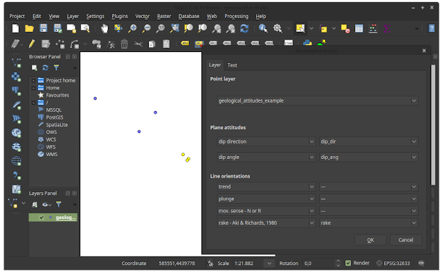
In the "Layer" tab of the input windows, you define the source fields for the different data types. Remember that definining (also) rake would override any data defined in the line orientation trend/plunge/movement sense fields.
 |
| Fig. 3. Definition of input fields for record dip direction, dip angle and rake angle. |
You define which type of data to plot for the "plot data" button. You could also previously have changed the default plot style via the "Plot style" button.
Here we plot faults with slickenlines. Also T-L diagrams are available.
 |
| Fig. 4. Choice of faults with slickenlines data type for stereonet plot. |
Et voilà..
 |
| Fig. 5. The stereonet of the faults and slickenlines data is displayed on the right. |
Clear the stereonet with "Clear stereonet". Obviously you can suporpose multiple plots into a single stereonet.
Save a figure with the tool from "Save figure" button.
To install the plugin, clone the repository or download and extract the zip file from https://github.com/mauroalberti/geocouche/releases in your local QGIS Python plugin folder (for instance: /home/mauro/.qgis2/python/plugins/geocouche) and activate the plugin in the installed section of QGIS "Manage and install plugins" command.
For any question: alberti.m65 at gmail.com
References
Aki, K., Richards P.G., 1980. quantitative Seismology Theory and Methods. Vol. I, W.H. Freeman and Company, San Francisco, CA,, 557 pp.
Alberti, M., 2005. Apllication of GIS to spatial analysis of mesofault population. Computers & Geosciences, 1249-1259.