GeoProfiler, porting of qProf to qgSurf

To create geological profiles, one of the available tools for QGIS is qProf. 

qProf is still maintained and features are added, mainly based on user requests and suggestions, but the main development has shifted to qgSurf, via the addition of the GeoProfiler tool, that is a porting of the functionalities of qProf to qgSurf.

 

 

GeoProfiler GUI is partially modified with respect to qProf and has a general workflow that surely has to be improved as easy of use but that should be more intuitive than that of qProf.

One of the main features of GeoProfiler is its ability to create parallel profiles, starting from a base one.

The following example illustrates the creation of parallel profiles.

We use a base profile, that corresponds to the blue dotted line in the figure below.

 

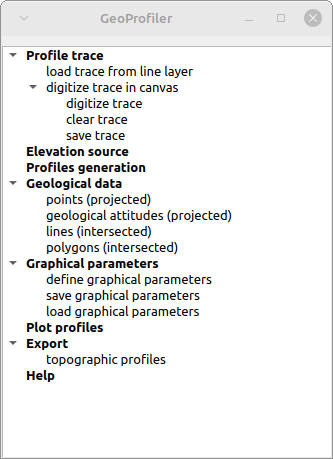
Having defined the base profile (in addition to the source DEM) we define the number and spacing of parallel profiles ('Profiles generation' command):

 

 

The tool automatically replicates the base profile 5 times, so that at the end we obtain parallel profiles as in the figure below.

  

 

The resulting profiles in plan view, with geological outcrops and fault line intersections, are obtained using the 'Plot profiles' command:

 

Important: to define and fine-tune the polygon and line intersections graphical parameters, as well to define the figure parameters, you need to find the best ones in the graphical parameters windows by trial-and-error.

Very important: defined polygon intersection will not show up in the profiles until you define their graphical parameters ('Polygon intersections' command in figure below).

 

 

Crucial: GeoProfiler has one major limitation, with respect to qProf: it does not handle source data with different CRS. So all input datasets must share the same CRS, say EPSG: 32633, to produce meaningful results.

The version of qgSuf with GeoProfiler included has been submitted to the QGIS plugin repository today (Nov. 27, 2022) and has yet to be approved. 

For the impatient or the curious, it can be downloaded and imported in QGIS as a zip file via the GitLab release (remember to unzip the downloaded file, rename the folder as "qgSurf", zip again with for instance 7Zip and install the plug-in from the new zip file)

 

Animations of geological profiles with map traces

 

In the new 6.2 pygsf release (2022/02/06) it is possible to create figures and also animations that represent a set of parallel profiles in which each geological profile is coupled with the related map trace.

Currently, the produced maps (left in the above animation) can only represent the profile traces, apart from the topography (optionally with a shaded relief). 

The code to create the above animation is available in the Jupyter notebook:

Geologic profiles map animations - the Timpa San Lorenzo structure (Southern Italy)

 

The release is available here:

https://gitlab.com/mauroalberti/gsf/-/tags/v6.2.0

Cross-section maps vs. profiles

 

The new pygsf release (v. 6.1.0) makes it possible to create and visualize directly in Jupyter, just using Python, topographic maps with superposed traces of parallel profiles, numbered by their ids as in the example below.

These map traces can be compared with the topographic vertical profiles displaying also geological information, for instance geological outcrops, that can be composed into an animation.

 

Next step would be to implement  the creation of animation with both the topographic vertical profile and a map with the corresponding map profile trace, so to make easier to relate each vertical profile with the related map trace.

The map traces and animation creations are detailed in this Jupyter notebook:

https://gitlab.com/mauroalberti/gsf/-/blob/master/docs/others/Geologic%20profiles%20-%20Timpa%20San%20Lorenzo.ipynb

 

The version 6.1.0 can be downloaded from:

https://gitlab.com/mauroalberti/gsf/-/tags/v6.1.0

Creating basic geological profile animations

In the new release (v. 6.0.0) of pygsf it is possible to create animations made up of parallel geological profiles.

An example is in the following gif:

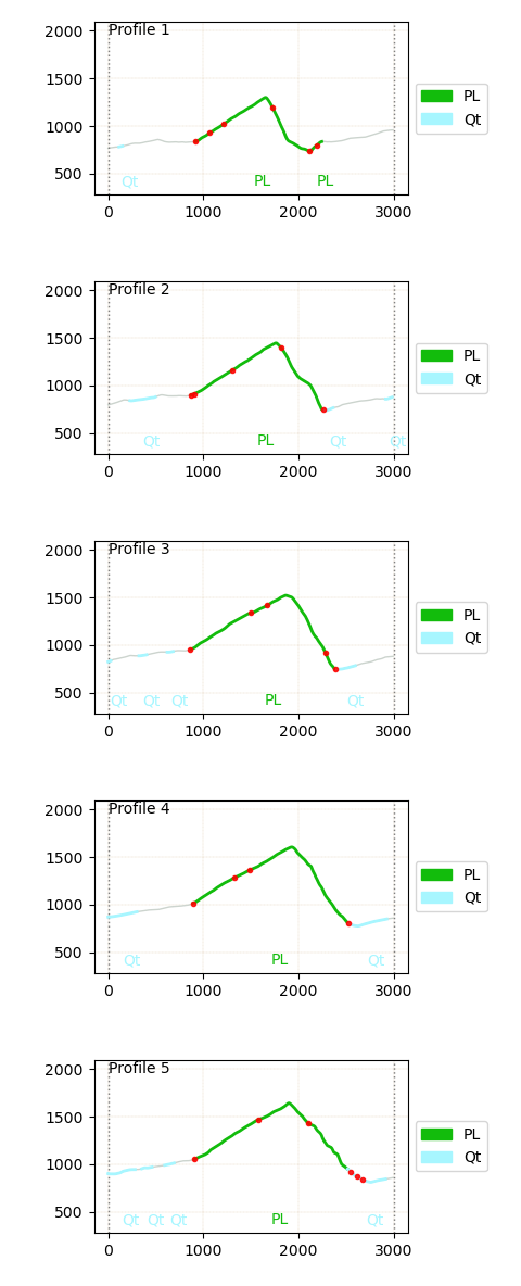
The red circles represent fault intersections, while the green thick lines (PL) are Mesozoic carbonatic outcrops and the grey ones (Qt) are Quaternary outcrops. The area is in Southern Apennines (Timpa di San Lorenzo carbonatic structure). The profiles are derived from a geological outcrop shapefile and a topographic DEM, both loaded in a Jupyter notebook using pygsf.

 

pygsf is a Python module (yet unpublished) for the processing of geological data.

The processing may be performed for instance in a Jupyter notebook.

The plan is to incorporate this module in a QGIS plugin, qgSurf, created for the processing of geological data.

For those interested, the animation derivation is detailed in this Jupyter notebook:

https://gitlab.com/mauroalberti/gsf/-/blob/master/docs/others/Geologic%20profiles%20-%20Timpa%20San%20Lorenzo.ipynb

 

The version 6.0.0 can be downloaded from:

https://gitlab.com/mauroalberti/gsf/-/tags/v6.0.0

 

Visualization and analyis of parallel topographic profiles in Jupyter

A new version (5.0.1) of pygsf adds tools for the creation and analysis of parallel profiles, for instance directly into a Jupyter notebook.

What is pygsf? It's a Python module devoted to the processing of topographic and geological data.

With the new tools, multiple profiles can be plotted, as well as their statistical properties: for instance the range of the profiles, their minimum, maximum and mean traces. The profiles can also be exported as a line shapefile, in order to visualize them in a GIS software (e.g. QGIS), or exported as an animated gif. 

The images below represent a brief tour of the methods available.

First is a simple plot of a single topographic profile.

We can create multiple parallel profiles, for instance 5 parallel profiles produced from the base profile using a user-provided normal offset:

The multiple profiles can be plotted into a single graph:

 

They can be composed into an animation (quite slow to play, I admit):

The minimum and the maximum of the profiles along the trace can be plotted in a single profile:

and also the range (maximum - minimum) calculated and plotted:

Last showed method  is the possibility to save the multiple profiles into a new line shapefile, that can be loaded for instance in QGIS to display the locations of the topographic sections created (the Mt. Alpi zone in the Lucania Southern Apennines, Italy):

 

 

 

 

The code repository is at:

https://gitlab.com/mauroalberti/gsf 

 

A quite detailed notebook describing how to reproduce the processing shown here is available at:

https://gitlab.com/mauroalberti/gsf/-/blob/master/docs/profiles/Topographic%20profiles%20with%20pygsf.ipynb

(note: unfortunately the embedded gif results broken) 

 

 

New release of qProf

qProf is a QGIS plugin for creating topographic and geological profiles.
A new version has been just released at: https://github.com/mauroalberti/qProf
This new version allows to create multiple topographic profiles, when the input profile lines are defined in a source line layer.
An example of a created profile is below.

To download the zipped plugin folder:

https://github.com/mauroalberti/qProf/releases

 Installation instructions are available at the main page:

https://github.com/mauroalberti/qProf

It's your fault

If you want to display your georeferenced faults in stereonets using QGIS you can use also the new functionalities in the geocouche plugin.

It uses apsg by Ondrej Lexa (apsg vers. 0.4.3 is incorporated in the plugin) for plotting geological data in stereonets. It allows to plot normal and reverse faults, while pure transcurrent faults are not explicitly treated in the used apsg version.

Input fault data format can follow two alternative formats:

1. slickenline dip trend and plunge, plus movement sense ("N" for normal faults and "R" for reverse faults)
2. rake angle according to the Aki & Richards (1980) convention (see Fig 1).

Fig. 1. Rake angle convention as defined from Aki & Richards (1980). Originally Figure 1 in Alberti (2005).

Take note that if you provide both line trend/plunge/movement sense and rake angle, rake angle takes precedence and shadows the data provided in the trend/plunge/movement sense format.

Now an example of using the geocouche tools for faults, using fault data stored in a point layer (this same layer is provided as a shapefile in the example data folder in the gihub repository).

You define the input data with the "Input data" button.  If you choose a (point) layer as source and there is a selection in the layer, only selected points will be considered.

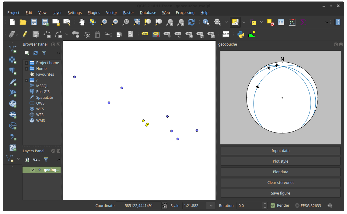
Fig. 2. Example data with three records selected in a point layer, plus, on the right, the geocouche plugin activated.

 In the "Layer" tab of the input windows, you define the source fields for the different data types. Remember that definining (also) rake would override any data defined in the line orientation trend/plunge/movement sense fields.

Fig. 3. Definition of input fields for record dip direction, dip angle and rake angle.

You define which type of data to plot for the "plot data" button. You could also previously have changed the default plot style via the "Plot style" button.
Here we plot faults with slickenlines. Also T-L diagrams are available.

Fig. 4. Choice of faults with slickenlines data type for stereonet plot.

Et voilà..

Fig. 5. The stereonet of the faults and slickenlines data is displayed on the right.

Clear the stereonet with "Clear stereonet". Obviously you can suporpose multiple plots into a single stereonet.
Save a figure with the tool from "Save figure" button.

To install the plugin, clone the repository or download and extract the zip file from https://github.com/mauroalberti/geocouche/releases in your local QGIS Python plugin folder (for instance: /home/mauro/.qgis2/python/plugins/geocouche) and activate the plugin in the installed section of QGIS "Manage and install plugins" command. 

For any question: alberti.m65 at gmail.com

 

References

Aki, K., Richards P.G., 1980. quantitative Seismology Theory and Methods. Vol. I, W.H. Freeman and Company, San Francisco, CA,, 557 pp.

Alberti, M., 2005. Apllication of GIS to spatial analysis of mesofault population. Computers & Geosciences, 1249-1259.

Plotting geological attitudes in stereonets using QGIS

A new plugin for QGIS, geocouche, allows to plot geological data attitudes stored in stereonets, using the plotting utilities provided by the apsg module by Ondrej Lexa. Data can be stored in geological layers or entered as text, and plotted as great circles or axis. The current release, as of April, 4th,  is vers. 1.0 and  can be downloaded from: https://github.com/mauroalberti/geocouche/releases

How it works? The following description derives from the tool help. 
With the current geocouche  release, it is possible:

1. to calculate the angles between planes stored in a layer and a reference plane
2. to plot data from layers or texts in stereonets

These two tools are available from the QGIS plugin interface.

Fig. 1. geocouche interface.

Geological angles

This tool allows to calculate the angles (as degrees) between a reference plane and the (eventually selected) features in a point layer (Fig. 2).

Fig. 2. Geological angles calculation interface.

It can be applied to determine the degree of misalignement between a reference (for instance, regional) measure and local geological measures.

Definition of parameters

The user has to define the two fields storing the azimuth (dip direction or RHR strike) and the dip angle of each feature, the attitude of the reference plane, and the name of the output shapefile with a new field storing the calculated angle (Fig. 3).

Fig. 3. Definition of parameters for angle calculation.

Geological stereonets

It allows to produce stereonets depicting geological plane and axis attitudes (Fig. 4). There are three steps:

1. Choice of input data
2. Definition of plot style
3. Data plotting

Fig. 4. Stereonet interface.

Choice of input data

It is possible to use input data from data stored in a point layer (Layer tab, Fig. 5) or to use text input (Text tab, Fig. 6).

Input from point layer

When using a point layer (already loaded in the TOC), plane and/or axis attitudes are defined via the fields storing their values (Fig. 5). When a selection is defined, only the selected features will be considered.

Fig. 5. Input from point layer interface.

Input from text

The input can be inserted into a text window (Fig. 6), defining if data consist of:

• planes

• axes

• planes and axes

Fig. 6. Input from text interface.

Another option to take care of, is,  for plane data, whether orientations are expressed using dip direction or RHR strike.

Plot style

Styles can be defined for both great circles and poles: color, width/size, line/marker style, and transparency (Fig. 7). Settings are stored in memory.

Fig. 7. Plot style interface.

Stereonet plotting

Plots can use a new or a pre-existing stereonet (provided it has not been previously closed) (Fig. 8).

Fig. 8. Stereonet plot interface.

Planes can be plotted as great circles or as plane normals, axes as poles or as normal great circles. An example of stereonet is shown in Fig. 9.

Fig. 9. Stereonet example.

A Linux tool for calculating local best-fit plane attitudes from geological traces

The topographic traces of geological surfaces store information on the 3D attitudes of the geological surfaces. Knowing the coordinates of the intersection points between a topographic surface and a geological surface, it is therefore possible to estimate the local attitudes of a geological surface.

 

The tools

 

A short description of geoSurfDEM: it is composed of two tools, IntersectDEM and the new BestFitGeoplanes.
The former allows to calculate the intersection points between a geological surfaces (stored in the VTK format) and a DEM. The latter, that will be described in the current post, allows to estimate the local attitudes given a set of 3D points, all deriving from the intersection between a single geological surface and a topographic surface. BestFitGeoplanes is developed using C++ and Fortran. The algorithm uses Singular Value Decomposition (SVD) in order to invert the local traces into local best-fit planes. 

The input data is constituted by a set of points (their x, y and z coordinates), all related to a single, continuous geological surface. How to process them in order to derive the local attitudes? Since the source points are unconnected points (not lines), all deriving from a single, continuous surface, the 2D space is discretized into a raster, using a user-defined cell size.
Based on the points falling into a cell, we have three possible cases:

1. no points falling into the cell;
2. one or two points falling into the cell;
3. three or more points in the cell.

In the first and second case, no attitude inversion via SVD is possible.
In the third case, when the points are not all collinear, a solution is provided by the SVD method. This solution is attributed to the grid cell.
The algorithm output will therefore consist in a gridded set of points for which the local attitudes have been inverted.
 
What is the difference with deriving the attitude via a spatial interpolation using for instance kriging? These interpolations implicitly assume a 2.5D surface and do not allow 3D surfaces. Geological surfaces, on the other hand, due to folding, can be 3D surfaces, i.e. with more then one point for each x-y position. Local inversion via SVD does not constrain the geological surfaces to be 2.5D,  but that may be locally modeled via a planar surface.

 

Compilation

 

This application is developed in Linux and is available at: https://github.com/mauroalberti/geoSurfDEM.
A makefile is available for compiling this tool in a Linux environment.
The compilation sequence is:
cd path/to/source/files
make
make clean

Lapack and BLAS libraries must be available. The makefile assumes that Lapack is available in usr/lib/lapack (with name lapack) and BLAS in usr/lib/libblas (name blas). Modify the makefile accordingly, to adapt to your settings. Alternatively, an example of commands to build it (always in a Linux environment and with same libraries settings) is in https://github.com/mauroalberti/geoSurfDEM/blob/master/BestFitGeoplanes/compile

 

Use

 

Having compiled the application, it is possible to run it as console application (Fig. 1). The only user interaction after launching the application is providing a parameter file name ("param.txt" in Fig. 1 example).

Fig. 1. Example of a run of the application.

 

The input parameter file is a text file that lists six pieces of information:

1. the path of text file storing the 3D coordinates (x, y and z) of the intersection points of a single, continuous, geological surface;
2. the number of header lines in the file referenced in point 1;
3. the path  of the text file in which the georeferenced results will be stored;
4. the path to the analysis report file;
5. the path of the output grid (in ESRI ASCII grid format) that will list the number of intersection points for each grid cell;
6. the output grid cell size;

 An example is available in https://github.com/mauroalberti/geoSurfDEM/tree/master/BestFitGeoplanes, in the param.txt file:

/home/mauro/Documents/Ricerca/Codice/Geostrutturale/geoSurfDEM/test_data/BestFitGeoplanes/inters_malpi_135_35.csv
1
/home/mauro/Documents/Ricerca/Codice/Geostrutturale/geoSurfDEM/test_data/BestFitGeoplanes/bfg_malpi_13535_100.txt
/home/mauro/Documents/Ricerca/Codice/Geostrutturale/geoSurfDEM/test_data/BestFitGeoplanes/rep_malpi_13535_100.txt
/home/mauro/Documents/Ricerca/Codice/Geostrutturale/geoSurfDEM/test_data/BestFitGeoplanes/pts_malpi_13535_100.asc
100 

The application output is represented by the three files listed in points 3-5 of the previous list. The more important is the inverted result file (point # 3), that consists in a csv file listing a few fields (see Fig. 2):

1. x: x coordinate of the cell grid center;
2. y: y coordinate of the cell grid center;
3. pt_num: number of points used for the inversion. Required minimum is 3.
4. dip_dir: inverted dip direction for geoplane points in cell;
5. dip_ang: inverted dip angle for geoplane points in cell;
6. x_range: spatial range along the x-direction (E-W) for the inverted points in the considered cell;
7. y_range: spatial range along the y-direction (N-S) for the inverted points in the considered cell;
8. z_range: spatial range along the z-direction (vertical) for the inverted points in the considered cell;
9. pseudo-volume: "pseudo"-volume defined by the inverted points in the cell, given by the product of the three previous ranges (i.e., x_range, y_range and z_range) - possibly removed in successive releases.

Fig. 2. Tabular view of the content of the inversion result file, as viewed by importing the file in QGIS.

 

A theoretical case study 

 

This post presents a practical assessment of the result, by using a theoretical surface for which the expected local attitudes are known (currently, as of February 2017, all example data are available at https://github.com/mauroalberti/geoSurfDEM/tree/master/test_data).
A theoretical plane has been generated using simSurf, with dip direction equal to 135° and dip angle of 35°.
This plane, saved in VTK format from within simSurf, has been used as input plane to be intersecated with a natural topographic surface, of the Mt. Alpi zone (Lucania, Southern Italy), using the IntersectDEM of geoSurfDEM.
The resulting intersection points are saved as a csv file, that can be used as input for the BestFitGeoplanes. The intersection points, to be used for the best-fit-plane local inversions, are represented in Fig. 3.

Fig. 3. Input points (yellow) representing the theoretical intersection between a geoplane oriented 135°/35° (dip dir. and dip angle) and a DEM topography (Mt. Alpi zone, Lucania, Southern Italy). Visualization using QGIS.

 

Using BestFitGeoplanes with the previously described param.txt file, we obtain a result that, for the georeferenced point part, imported in QGIS is shown in Fig. 4.

Fig. 4. The same as in Fig. 3, plus superposed the gridded points with inverted results (orange dots). Visualization with QGIS.

 

How much the inverted results conform to the theoretical input source, that as said is a plane with a dip direction of 135° and a dip angle of 35°?
A stereoplot, created with the geocouche plugin for QGIS, illustrates the degree of  concordance between the source attitude (135°/35°, blue great circle in Fig. 5) and the inverted local attitudes (semi-transparent orange great circles in Fig. 5).
The majority of inverted data conform closely to the expected result, while a few inversions show a minor deviation from the expected result.

 

Fig. 5. Stereonet representing the inferred local plane attitudes as semi-opaque orange great circles, and the source geological plane attitude (135°/35°) as blue great circle. Created with geocouche.

The deviations of the inverted results from the expected value were calculated using the "Geological angles" of geocouche and the statistics calculated with QGIS (see Fig. 6). The maximum is 9.3° and the minimum almost zero, while the median and mean deviation values are lower than 0.5°. The standard deviation is about 1.2°. So in general we can be quite confident in the generated results. More in-depth analyses of the deviations of expected-versus-inferred results could be the subject of a still to-be-written paper.

Fig. 6. Statistics for angular deviations of the calculated results from the theoretical test case.

Edits

2022-12-29: improved paragraph styling; modified input parameters description (items 5 and 6)

geoSurfDEM: a C++ console application for determining intersections between 3D geological surfaces and topography

The determination of the theoretical intersections between digital 3D geological surfaces and topography could be of potential help for studying the field attitudes of natural geological surfaces, as mapped from outcrops or from aerial and satellite images. Since geological structures have complex geometries, the analysis of the relationships between 3D surfaces and topography requires tools that can process 3D geological surfaces.

geoSurfDEM aims at determining:

a) the theoretical intersections between a 3D surface and a topography
b) the local 3D attitude of that surface at each intersection point

How does it work?

Below you see the screenshot of an application run in a Linux shell. When compiled for Windows, the procedure is identical. The total run time can be quite long, many minutes or more.

What is to note?

After the application header display, the user is asked for the name of a text file. In this example, "input_files.txt" is provided, the name of a file located in the same directory as the running application. This file provides the paths of three files:

1) DEM, in ESRI ASCII grid format
2) geological surface, in (old) VTK text format
3) output csv file storing for each row: x-y-z-dip direction-dip angle

An example of input text file is the following:

./publ_data/dem_malpi_aster_wgs84utm33.asc
./publ_data/geological_plane.vtk
./publ_data/intersections.csv


Examples of input data files (i.e., DEM ASCII grid, VTK geosurface file, CSV intersection result) are present in the publ_data subdirectory.

Afterwards, the application outputs a few informative messages about the number of found features and at the last prints out the number of found intersecting points, hopefully greater than zero. The results are stored in the text file referenced by the third path in the input text file.

Example of use

To present the application and check the validity of its results, we use a theoretical test case, i.e. a geological plane with a desired attitude 135°/35°, and with a spatial extent fitting that of the test DEM, covering the Mt. Alpi zone (Basilicata, Southern Italy), derived from global ASTER data.
You can export a DEM in ESRI ASCII grid format with Saga GIS (in addition to ArcGIS).

Creation of test geological plane

The geological plane is created and saved as a VTK text file with simSurf. With this Python 2.7 tool, it is possible to simulate geological surfaces by using analytical formulas.

simSurf is subdivide in two modules:

a) geosurface_simulation.py: creates, geolocates and saves/exports an analytical surface
b) geosurface_deformation.py: reads an analytical surface created by the previous module, deforms it and saves/exports.

Horizontal plane creation

So we start creating a horizontal plane with the Geosurface simulation tool, Analytical formula part, see figure below.

The zero in the formula section is for the horizontal plane creation. You calculate the matrix and you can see the plane in three dimensions.

Then to the geographical parameters, that have to fit the DEM extent without creating an excessively large geological plane.

We create the simulated geosurface, optionally view it in three dimensions and then have to export it in the Geo Analytical Surface (GAS) format, i.e. a jason format.

Plane rotation

We then pass to the Geosurface deformation tool, import the previously exported jason file and then apply a rotation to the plane around a N-S horizontal axis, by 35°.

Apply and then rotate by 45° around a vertical axis (plunge equal to 90°).

In this way we obtain a plane dipping 35° towards N135°.

Plane displacement to DEM extent

Now we locate the rotated plane to a geographical position that broadly fits with the DEM. I choose to use my qgSurf plugin for QGIS for quickly locating a point at the center of the used DEM, while knowing also the z value.

You see to the right the coordinates (x-y-z) of the point at the DEM center, showed within QGIS.

I copied and pasted these values in the simSurf displacement tab, so that the plane is displaced by the given delta-x, delta-y and delta-z amounts.

Done, after applying.


Save the geosurface as a VTK file and then you can see it in Paraview and use in the geoSurfDEM application. Note that the VTK file stores the plane as triangle mesh, without explicit attitude (i.e., dip direction and angle) information. So the local results calculated by the geoSurfDEM application are derived by the local geosurface triangle attitude stored in the VTK file. Using a simple plane obviously we expect the same results for all intersection points.

Input data preview

We see how are the DEM and the VTK plane data in Paraview.

You can import the DEM when in x-y-z format (could create with Saga), then applying a
Table to Point filter, while the VTK format is directly read from Paraview. Here a nadiral view.
Y axis represents the North.

And a lateral one, as seen from the South.

geoSurfDEM result

At the end, what are the results of the geoSurfDEM application?

We see them displayed in Paraview, by importing the resulting csv file and superposing on the DEM points and the plane surface. The results are symbolized by blue dots. You see them following the visual intersection between the plane with dip direction 135° and dip angle 35° and the DEM.

 

Always in Paraview we see, for a few records, that the corresponding point attitudes calculated by geoSurfDEM are as expected: 135°/35° for each point, since in this test case we were dealing with a geological plane.

----------

The code repository of geoSurfDEM is at https://gitlab.com/mauroalberti/geoSurfDEM

Executables for Linux are also availables for Linux (64 bit) at the code repository.

EDITS: 

2023-01-01: fixed broken llinks to images

Adding a Python module to QGIS Python in Windows with multiple Python installations

Both Python and (if I rememeber well) QGIS were originally created for Linux. Their use in Windows is somewhat complicated by the difficulties to adapt these tools to a different environment.
When working with an installation of QGIS in Windows created with the standalone installer, one may need to use Python modules that are not present in the default QGIS installation. Modules are generally installed in the folder ..\Python27\Lib\site-packages.
The installation can be confusing if you have also other Python installations, for instance one derived from the Python(x,y) distribution, from Anaconda or from ArcGis.
The QGIS Python installation from the standalone GGIS installer is not system-wide, and QGIS Python is separated and independent from the other Pythons.
After a bit of struggling, I found a way to install a Python module from the source files (tar.gz) in QGIS Python.

Source module

The Python module that I wanted to install is pyserial, that I downloaded as a tar.gz file from https://pypi.python.org/pypi/pyserial.
I uncompressed it in a temp folder, in my particular case:
C:\Temp\dist\pyserial-2.7\pyserial-2.7
This folder contains the required setup.py file, plus some other stuff.

Target QGIS installation 

The target QGIS installation is 2.10.1 Pisa 32bit (from standalone installer), with installation folder:
C:\Program Files (x86)\QGIS Pisa

In QGIS Python, the path to the standard Python module folder is:
..\QGIS Pisa\apps\Python27\Lib\site-packages.
Installing a module in this last directory, we have it recognized by QGIS Python.

Prerequisites

As a prerequisite, you have to be sure to launch from the DOS shell the QGIS Python and not other Python interpreters. To achieve that, one possible (but there are others) way is to add the path to the QGIS python.exe file as the first item in the system PATH.
In Windows 8, follow Control Panel -> System and Security -> System and then , by opening Advanced system settings, modify the Path variable (user or system are equivalent ways, I suppose, in my case I had the system one modified) by adding as the first voice:
C:\Program Files (x86)\QGIS Pisa\bin
i.e., the bin folder of the QGIS installation, where python.exe is contained.

Procedure

Being sure that from the DOS shell you are invoking the QGIS Python, you can then proceed as follows:

1) launch an administrator dos shell, to be sure to have write permissions in the target directory

2) in the dos shell, change directory to the uncompressed folder of the new module to install, (it should contain the setup.py file), in my case with the command:
  cd C:\Temp\dist\pyserial-2.7\pyserial-2.7

3) always in the dos shell, run the python setup.py install command on the module, in my case:
  python setup.py install --prefix="\Program Files (x86)\QGIS Pisa\apps\Python27"
Change path in the prefix option accordingly to your particular QGIS installation. Note two things:

• do not put the drive character at the beginning of the prefix path; 
• point to the Python27 folder, not to the  Python27\Lib\site-packages

Checking the results

In addition to the installation messages in the DOS shell, that should present no errors, you may then check that the module installation was successful by trying to import the specific module in the QGIS Python console, in my case:
import serial
You should receive no import error messages..