geoSurfDEM: a C++ console application for determining intersections between 3D geological surfaces and topography

The determination of the theoretical intersections between digital 3D geological surfaces and topography could be of potential help for studying the field attitudes of natural geological surfaces, as mapped from outcrops or from aerial and satellite images. Since geological structures have complex geometries, the analysis of the relationships between 3D surfaces and topography requires tools that can process 3D geological surfaces.

geoSurfDEM aims at determining:

a) the theoretical intersections between a 3D surface and a topography
b) the local 3D attitude of that surface at each intersection point

How does it work?

Below you see the screenshot of an application run in a Linux shell. When compiled for Windows, the procedure is identical. The total run time can be quite long, many minutes or more.

What is to note?

After the application header display, the user is asked for the name of a text file. In this example, "input_files.txt" is provided, the name of a file located in the same directory as the running application. This file provides the paths of three files:

1) DEM, in ESRI ASCII grid format
2) geological surface, in (old) VTK text format
3) output csv file storing for each row: x-y-z-dip direction-dip angle

An example of input text file is the following:

./publ_data/dem_malpi_aster_wgs84utm33.asc
./publ_data/geological_plane.vtk
./publ_data/intersections.csv


Examples of input data files (i.e., DEM ASCII grid, VTK geosurface file, CSV intersection result) are present in the publ_data subdirectory.

Afterwards, the application outputs a few informative messages about the number of found features and at the last prints out the number of found intersecting points, hopefully greater than zero. The results are stored in the text file referenced by the third path in the input text file.

Example of use

To present the application and check the validity of its results, we use a theoretical test case, i.e. a geological plane with a desired attitude 135°/35°, and with a spatial extent fitting that of the test DEM, covering the Mt. Alpi zone (Basilicata, Southern Italy), derived from global ASTER data.
You can export a DEM in ESRI ASCII grid format with Saga GIS (in addition to ArcGIS).

Creation of test geological plane

The geological plane is created and saved as a VTK text file with simSurf. With this Python 2.7 tool, it is possible to simulate geological surfaces by using analytical formulas.

simSurf is subdivide in two modules:

a) geosurface_simulation.py: creates, geolocates and saves/exports an analytical surface
b) geosurface_deformation.py: reads an analytical surface created by the previous module, deforms it and saves/exports.

Horizontal plane creation

So we start creating a horizontal plane with the Geosurface simulation tool, Analytical formula part, see figure below.

The zero in the formula section is for the horizontal plane creation. You calculate the matrix and you can see the plane in three dimensions.

Then to the geographical parameters, that have to fit the DEM extent without creating an excessively large geological plane.

We create the simulated geosurface, optionally view it in three dimensions and then have to export it in the Geo Analytical Surface (GAS) format, i.e. a jason format.

Plane rotation

We then pass to the Geosurface deformation tool, import the previously exported jason file and then apply a rotation to the plane around a N-S horizontal axis, by 35°.

Apply and then rotate by 45° around a vertical axis (plunge equal to 90°).

In this way we obtain a plane dipping 35° towards N135°.

Plane displacement to DEM extent

Now we locate the rotated plane to a geographical position that broadly fits with the DEM. I choose to use my qgSurf plugin for QGIS for quickly locating a point at the center of the used DEM, while knowing also the z value.

You see to the right the coordinates (x-y-z) of the point at the DEM center, showed within QGIS.

I copied and pasted these values in the simSurf displacement tab, so that the plane is displaced by the given delta-x, delta-y and delta-z amounts.

Done, after applying.


Save the geosurface as a VTK file and then you can see it in Paraview and use in the geoSurfDEM application. Note that the VTK file stores the plane as triangle mesh, without explicit attitude (i.e., dip direction and angle) information. So the local results calculated by the geoSurfDEM application are derived by the local geosurface triangle attitude stored in the VTK file. Using a simple plane obviously we expect the same results for all intersection points.

Input data preview

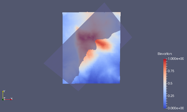
We see how are the DEM and the VTK plane data in Paraview.

You can import the DEM when in x-y-z format (could create with Saga), then applying a
Table to Point filter, while the VTK format is directly read from Paraview. Here a nadiral view.
Y axis represents the North.

And a lateral one, as seen from the South.

geoSurfDEM result

At the end, what are the results of the geoSurfDEM application?

We see them displayed in Paraview, by importing the resulting csv file and superposing on the DEM points and the plane surface. The results are symbolized by blue dots. You see them following the visual intersection between the plane with dip direction 135° and dip angle 35° and the DEM.

 

Always in Paraview we see, for a few records, that the corresponding point attitudes calculated by geoSurfDEM are as expected: 135°/35° for each point, since in this test case we were dealing with a geological plane.

----------

The code repository of geoSurfDEM is at https://gitlab.com/mauroalberti/geoSurfDEM

Executables for Linux are also availables for Linux (64 bit) at the code repository.

EDITS: 

2023-01-01: fixed broken llinks to images

Adding a Python module to QGIS Python in Windows with multiple Python installations

Both Python and (if I rememeber well) QGIS were originally created for Linux. Their use in Windows is somewhat complicated by the difficulties to adapt these tools to a different environment.
When working with an installation of QGIS in Windows created with the standalone installer, one may need to use Python modules that are not present in the default QGIS installation. Modules are generally installed in the folder ..\Python27\Lib\site-packages.
The installation can be confusing if you have also other Python installations, for instance one derived from the Python(x,y) distribution, from Anaconda or from ArcGis.
The QGIS Python installation from the standalone GGIS installer is not system-wide, and QGIS Python is separated and independent from the other Pythons.
After a bit of struggling, I found a way to install a Python module from the source files (tar.gz) in QGIS Python.

Source module

The Python module that I wanted to install is pyserial, that I downloaded as a tar.gz file from https://pypi.python.org/pypi/pyserial.
I uncompressed it in a temp folder, in my particular case:
C:\Temp\dist\pyserial-2.7\pyserial-2.7
This folder contains the required setup.py file, plus some other stuff.

Target QGIS installation 

The target QGIS installation is 2.10.1 Pisa 32bit (from standalone installer), with installation folder:
C:\Program Files (x86)\QGIS Pisa

In QGIS Python, the path to the standard Python module folder is:
..\QGIS Pisa\apps\Python27\Lib\site-packages.
Installing a module in this last directory, we have it recognized by QGIS Python.

Prerequisites

As a prerequisite, you have to be sure to launch from the DOS shell the QGIS Python and not other Python interpreters. To achieve that, one possible (but there are others) way is to add the path to the QGIS python.exe file as the first item in the system PATH.
In Windows 8, follow Control Panel -> System and Security -> System and then , by opening Advanced system settings, modify the Path variable (user or system are equivalent ways, I suppose, in my case I had the system one modified) by adding as the first voice:
C:\Program Files (x86)\QGIS Pisa\bin
i.e., the bin folder of the QGIS installation, where python.exe is contained.

Procedure

Being sure that from the DOS shell you are invoking the QGIS Python, you can then proceed as follows:

1) launch an administrator dos shell, to be sure to have write permissions in the target directory

2) in the dos shell, change directory to the uncompressed folder of the new module to install, (it should contain the setup.py file), in my case with the command:
  cd C:\Temp\dist\pyserial-2.7\pyserial-2.7

3) always in the dos shell, run the python setup.py install command on the module, in my case:
  python setup.py install --prefix="\Program Files (x86)\QGIS Pisa\apps\Python27"
Change path in the prefix option accordingly to your particular QGIS installation. Note two things:

• do not put the drive character at the beginning of the prefix path; 
• point to the Python27 folder, not to the  Python27\Lib\site-packages

Checking the results

In addition to the installation messages in the DOS shell, that should present no errors, you may then check that the module installation was successful by trying to import the specific module in the QGIS Python console, in my case:
import serial
You should receive no import error messages..

beePen: a tool for drawing freehand annotations in QGis

beePen is an experimental Python plugin for drawing freeand annotations and sketches in an ad-hoc layer in QGis. It is inspired by the corresponding tool in BeeGIS and re-use the code by Pavol Kapusta in his Frehand Editing plugin.

beePen allows to create an annotation layer, that is characterized by three fields, storing the user-defined width, color and transparency of the pen. These value are automatically inserted based on the user choice in the plugin window (Fig. 1).

Fig. 1

To draw annotations, first you have to open the beePen window with the "bee" command (see Fig. 2, second icon from the right), eventually create a new annotation layer from the beePen window (see Fig. 1) or use an old one, put in edit mode using the standard tool of QGis (command at the left in Fig. 2) and then draw after selecting the pen tool (rightmost command in Fig. 2).

Fig. 2

The conception of beePen is by Mauro Dedonatis (Urbino Univ., Italy), while the implementation is by Mauro Alberti.

Some minor enhancements in qProf

qProf is a QGIS plugin for the creation of topographic and geologic profiles. Some minor enhancements were added to qProf in the new, experimental releases 0.2.9 and 0.3.0.

In version 0.2.9 the following options were added:
- the calculation of the absolute slope along the profile; previously only the directional slope was calculated;
- the possibility to flip a profile horizontally (option "Reverse profile direction"), as well as to reverse the orientation of the x axis (option "Reverse x axes direction) were added.

See examples in Figs. 1-4 (below).

Fig. 1. Map of Mt. Alpi zone (Basilicata, Southern Italy), with profile in red (direction from left to right). DEM data: TINITALY.

Fig. 2. Topographic (top) and absolute slope (bottom) profiles (see map trace in Fig. 1).

Fig. 3. Same profile as in Fig. 2, but with profile direction reversed.

Fig. 4. Same profile as in previous figures, but with reversed x axes directions.

In version 0.3.0, released on 2015-03-08, the possibility of configuring the figure save parameters (width, resolution, font size, subplot configuration parameters) was added. These graphic parameters can be saved in a text file and subsequently loaded for being applied to future plots.
This option is available from Export - Figure. Fig. 5 represents the window for defining the parameters, saving or loading them, and also for saving the figure as a file in PDF, SVG or TIF formats.

Fig. 5. Window for saving a figure as a graphic file, and for configuring graphic parameters, and saving or loading them.

The two versions are experimental since the impact of reversing the profile on the geological plotting has not been fully tested. For geological plots, the suggested version is 0.2.8.

Gerrit Tombrink, PhD student at the Goettingen University (Germany), is thanked for proposing the implemented options.

Cross-section intersections of line and polygon layers with qProf in QGis

A new release of qProf, plugin for QGis, allows to determine the intersections of line and polygon layers, representing for instance faults and geological outcrops, on a vertical cross-section.
These new functionalities complement those already available for projecting geological attitudes and lines on a cross-section.
The resulting data can be saved as shapefiles and csv.

Example of cross-section representing geological polygon layer intersections with a topographic profile.

The plugin can be installed/updated via the plugin manager of QGis. Alternatively it can be downloaded from the QGis plugin repository:
http://plugins.qgis.org/plugins/qProf/
or from the Bitbucket repository:
https://bitbucket.org/mauroalberti/qprof/downloads

R is progressing fast in TIOBE Index

According the TIOBE Index for November 2014, R, an open source statistical language,  progressed from position 15 in October to position 12 in November, thus heading for entering in the "top 10". It is preceded by Visual Basic and Visual Basic .NET. For instance, Python is at position 7.
The much younger Julia language is at position 126 while MATLAB is # 24.
More details:
http://www.tiobe.com/index.php/content/paperinfo/tpci/index.html

Changes in qgSurf plugin tools

Due to persisting plugin incompatibilities, related to Matplotlib, I've created a new qgSurf version, # 0.3.4. This version is made up by just two tools: "Best fit plane" and "DEM-plane intersection".
The removed 3D surfaces simulation and deformation tools are now available in a pure Python project, "simSurf", developed and tested in Linux Mint and published at: https://github.com/mauroalberti/simSurf.

Simulation and deformation of georeferenced geological surfaces: a pure Python implementation

A pure Python project for simulation and deformation of georeferenced geological surfaces is presented at:
https://github.com/mauroalberti/simSurf
It is an updated and Python-based, independent version of the simulation and deformation modules originally presented in the qgSurf plugin (vers. 0.3.3) for Quantum GIS. It is developed and tested in Linux Mint.
Two modules, "geosurface_simulation.py" and "geosurface_deformation.py" make possible to simulate and deform georeferenced surfaces (see example in Fig. below).

Example of a sheared and rotated sinusoidal surface with geographic parameters matching those of the Mt. Alpi - Mt. Raparo Aster DEM (Lucania, Southern Italy). The view is from NE to SW. Mt. Raparo is at the right. 3D visualization created with ArcScene (ESRI).

A MOOC on Numerical Methods with Python, starting August 18, 2014

A new MOOC, "Practical Numerical Methods with Python", with Lorena A. Barba and other instructors, has just started.
The link is: http://openedx.seas.gwu.edu/courses/GW/MAE6286/2014_fall/about

New version of qgSurf for QGIS

A new version of qgSurf, 0.3.3, has been released. It adds the possibility to use point or line layers as sources for the best-fit-plane calculation.
The plugin should work also in QGIS 2.2.0 for Windows 8 - 64 bit, even if the QGIS installer complains about a lacking dependency, Tkinter, a problem that I will investigate in the next days. If however you accept the installation, close QGIS and then reopen it, QGIS will present the plugin as installed and available. No problem of this kind has been observed in Windows Vista and Ubuntu.

Backward pathline calculation for steady vector fields in Quantum GIS

Calculating backward pathlines in steady vector fields is possible using the new version of VectorFieldCalc, a Python plugin for Quantum GIS. The pathline calculation is implemented via the Runge-Kutta-Fehlberg method (see references at the end).

For forward calculations, the user defines positive values of time steps and total times. For backward calculations, use negative values for both total time and time steps. An example for the last case, using the example data provided in the plugin folder, is below.

The result of the backward pathline calculation is presented in the figure below, with pathline points symbolised by increasingly negative total time, together with labels of the total times. The flows in this Antarctic glacier in Terra Nova Bay (data from D. Biscaro PhD thesis) are from top-left to bottom-right. Higher velocities of the flow field are in red, lower velocities in blue. Starting points are represented by red squares in the bottom-left section of the glacier.

 The plugin can be installed via the usual procedure for Quantum GIS, using the plugin manager.

For additional details (based on the previous version) you can see:
- Vector Field Processing
- 'Vector field processings': un plugin Quantum GIS per l'analisi di campi vettoriali 2D (in Italian)

Released first beta version of gvSIG CE 1.0.0 (64 bit OS)

From gvSIG CE developer announcement:

The first beta version of gvSIG CE 1.0.0 has just been released.
Downloads for Linux, Mac OS X and Windows here:
https://sourceforge.net/projects/gvsigce/files/beta-1/
All provided packages are for 64 bit operating systems.

Read the full announcement at:
http://gvsigce.sourceforge.net/wiki/index.php/GvSIG_CE_1.0.0_beta_1_release_notes

Plot of geological attitudes and traces in vertical sections along fold axes with Quantum GIS and qProf

The new released version of qProf (0.2.4), a Python plugin for Quantum GIS, allows to project geological attitudes and traces onto a vertical section along fold axes. On-the-fly reprojection of layers is supported.

The first step in using this plugin is creating a topographic profile by defining one (or more) source DEMs and a line layer that define the section, plus a line densify distance (generally of the order of the used DEM cell resolution) and an optional line order field (required only when the input geometry of the line layer is not sufficiently simple, see previous posts on the qProf plugin).
While for creating only topographic profiles the input line can be made up of many points and more than one DEM can be used, for geological projections the input line must be made up by just two points and only one DEM may be selected.
After having defined and created the profile using the tools in the "profile" tab, it is then possible to project geological attitudes or traces by using the commands in the "Project" tab.


Projection of geological attitudes

Geological attitudes will be stored in a point layer, with the measured dip direction and dip angle of the features in two distinct fields of the attribute table.
The commands are available from the "Geological attitudes" subwindow.
The projection of geological attitudes may be applied via different methodologies: (a) the nearest intersection point between the geological plane of a feature and the section plane; (b) using a common projection ("fold") axis for all features; (c) using individual axes for each attitude, with two numeric fields storing trend and plunge values.
If some data are selected, only those selected will be plotted, otherwise all layer features will be used. Labels can also be added to projected measures.
It is possible to cumulate in a single analysis session more sub-analyses, distinguishing them via different colors. Previous sub-analyses can be removed with the 'Reset geological attitudes' button.
Data can be saved as csv files or shapefiles.

A plot example, with attitudes labelled by original trend and plunge values, is in the figure below.

Projection of line traces

Line traces can represent the intersection of geological surfaces with the topography. When these surfaces are cylindrically folded, it is possible to projected the traces onto the section via a user-defined fold axis. The elevation information will be derived from the chosen DEM.
The commands are available from the "Geological traces" subwindow.
A line layer has to be chosen, with the name of the id field and a value for the line densification.
Trend and plunge of the projection axis will be defined, and a color chosen for the line plotting.
Different subanalyses, with different projection axes, can be differentiated by using different colors.
Previous analyses can be eliminated with the "Reset traces" command.
Results can be saved as text file, storing id-s-z values (where s is the horizontal distance from the section start) for each resulting point.

An example of the output is below. In this case, only geological traces are plotted. In general, both geological traces and attitudes can be plotted in the same section.

Installation

qProf can be installed from Quantum GIS via the plugin manager, or downloaded and unzipped in the Python plugin folder from:

• Quantum GIS  plugin repository: https://plugins.qgis.org/plugins/qProf/version/0.2.4/
• BitBucket: https://bitbucket.org/mauroalberti/qprof/downloads 

For bug segnalation:

• https://bitbucket.org/mauroalberti/qprof/issues?status=new&status=open

or write directly to alberti.m65@gmail.com (also for improvement requests or questions).